All You Need to Know About Maximum Likelihood Estimation

This post was originally published on Medium on June 21, 2018. View original article.

Probability Basics

Probability is the chance of an event $A$ occurring out of all possible events in the sample space $S$:

\[P(A) = \frac{|A|}{|S|}\]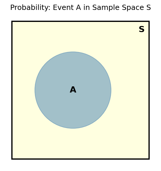

Joint Probability

Joint probability is when multiple events occur at the same time. For events $A$ and $B$:

\[P(A, B) = \frac{|A \cap B|}{|S|}\]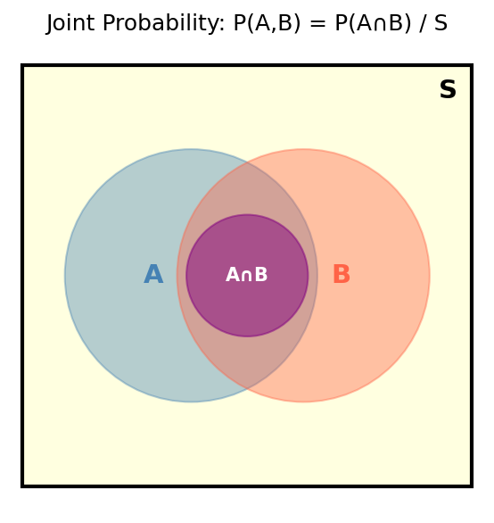

Conditional Probability

Conditional probability is the probability of event $A$ occurring, given that event $B$ has already occurred. Here, $B$ becomes our new sample space:

\[P(A \mid B) = \frac{P(A \cap B)}{P(B)}\]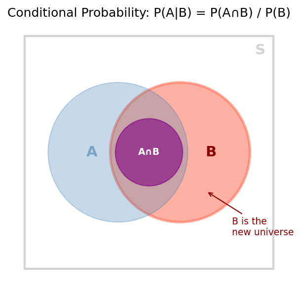

Bayes’ Rule

Starting from conditional probability, we can derive Bayes’ rule:

\[P(A \mid B) = \frac{P(B \mid A) \cdot P(A)}{P(B)}\]

Or put another way:

\[\text{Posterior} = \frac{\text{Likelihood} \times \text{Prior}}{\text{Evidence}}\]

Bayes’ rule lets us compute the probability of something happening based on what we’ve already observed, which is why it shows up everywhere in Bayesian inference.

Probability Distribution

A probability distribution is a function that tells you the probability of each value a random variable can take. Some common ones are the Gaussian (normal) distribution, the binomial distribution, and the beta distribution.

Every distribution has a set of parameters $\Theta$ that define its shape. For a Gaussian, those are the mean $\mu$ and the variance $\sigma^2$.

Maximum Likelihood Estimation

Say we have a dataset $X = {x^{(1)}, x^{(2)}, \ldots, x^{(n)}}$ that we believe was drawn from some distribution with parameters $\Theta$. We don’t know what $\Theta$ is. The idea behind Maximum Likelihood Estimation (MLE) is simple:

Find the parameter values $\Theta^*$ that make the data we observed as likely as possible under the distribution.

The Likelihood Function

If we assume the data points are independent and identically distributed (i.i.d.), then the likelihood of seeing the whole dataset is just the product of the likelihoods of each individual point:

\[L(\Theta \mid X) = \prod_{t=1}^{n} p(x^{(t)} \mid \Theta)\]

Log-Likelihood

Multiplying a lot of small probabilities together is a bad idea on a computer, the result quickly underflows to zero. To get around this, we take the log. Since $\log$ is monotonically increasing, the $\Theta$ that maximizes the log-likelihood is the same $\Theta$ that maximizes the likelihood:

\[\ell(\Theta \mid X) = \sum_{t=1}^{n} \log p(x^{(t)} \mid \Theta)\]

The product becomes a sum, which is much nicer to work with.

Finding the Optimal Parameters

Now we just need to maximize the log-likelihood:

\[\Theta^* = \arg\max_{\Theta} \; \ell(\Theta \mid X) = \arg\max_{\Theta} \sum_{t=1}^{n} \log p(x^{(t)} \mid \Theta)\]

For some distributions like the Gaussian, you can solve this by hand, take the derivative with respect to $\Theta$, set it to zero, and solve for $\Theta$. For more involved models, we fall back on gradient-based optimization.

MLE shows up all over machine learning. It’s the idea behind logistic regression, Gaussian mixture models, and the training objective for a lot of neural networks.