Logistic Regression in a Nutshell

This post was originally published on Medium on June 29, 2018. View original article.

Get ready to classify some data!

Logistic regression is a supervised ML algorithm. A bit of calculus, probability, and statistics will go a long way here.

Problem Setup

Say we have a training dataset with binary labels (0 or 1). We want to train a model that tells us the probability of a sample belonging to the positive class.

So the model learns weights $W$ to compute $P(y = 1 \mid W, X)$.

Likelihood Function

The likelihood for a single training sample is:

\[h^y \times (1 - h)^{(1 - y)}\]

where $h$ is the model’s prediction, the probability it assigns to the sample being in the positive class.

Log-Likelihood Objective

We maximize the log-likelihood over the whole training set:

\[\ell(W) = \sum_{i=1}^{n} \left[ y^{(i)} \log h(x^{(i)}) + (1 - y^{(i)}) \log \left(1 - h(x^{(i)})\right) \right]\]

Taking the log turns the product over samples into a sum, which is much nicer to work with when we start differentiating.

Decision Boundary Development

We could try modeling $p$ as a linear function of $X$ directly, but $p$ is stuck between 0 and 1 and linear functions aren’t. So instead, we work with the log-odds (or logits):

\[\log\left(\frac{p}{1 - p}\right)\]

This quantity is free to roam from $-\infty$ to $+\infty$, which is exactly what a linear function needs. So we set:

\[\log\left(\frac{p}{1 - p}\right) = W \cdot X\]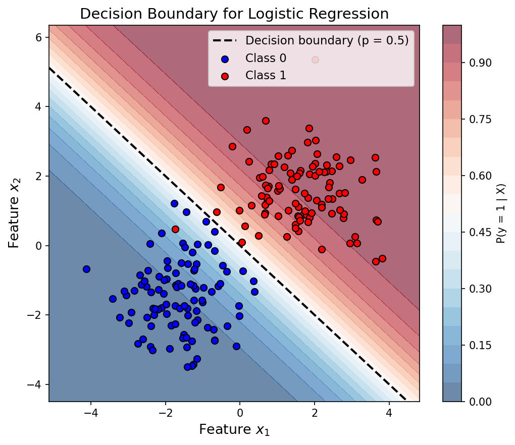

The Sigmoid Function

Now just solve the log-odds equation for $p$, and out pops the sigmoid (aka logistic) function:

\[p = \sigma(W \cdot X) = \frac{1}{1 + e^{-W \cdot X}}\]

It squashes any real number into a probability between 0 and 1. Neat.

Classification Rule

Once we have $p = \sigma(W \cdot X)$, classifying a sample is straightforward:

Condition	Prediction
$p > 0.5$	Positive class ($y = 1$)
$p < 0.5$	Negative class ($y = 0$)
$p = 0.5$	Decision boundary

Optimization

To maximize the log-likelihood, Newton’s method works really well. The update rule is:

\[W \leftarrow W - H^{-1} \nabla_W \ell(W)\]

where $H$ is the Hessian, the matrix of second-order partial derivatives of $\ell(W)$.

Since Newton’s method uses curvature information on top of the gradient, it tends to converge in way fewer iterations than plain gradient descent. The tradeoff is that you have to compute and invert the Hessian at every step.