Gradient Descent: Backbone of Most Popular Machine Learning Algorithms

This post was originally published on Medium on June 18, 2018. View original article.

Introduction to Machine Learning

Before I get into gradient descent, let me quickly walk through how I think about machine learning. Almost every ML algorithm boils down to four steps:

1. Define a model
2. Make predictions on the training data
3. Calculate the prediction error
4. Tune the model’s weights to reduce that error

That last step is where gradient descent comes in, and it’s honestly the step that matters most. You can have the fanciest model in the world, but if you can’t optimize its weights properly, it won’t learn anything useful.

What is Gradient Descent?

Gradient descent is by far the most popular optimization algorithm in machine learning. It’s a first-order optimization algorithm, which just means it only uses the first derivative (the gradient) to figure out which direction to move. In this post I’ll stick to Batch Gradient Descent, where we compute the gradient over the entire training dataset at each step.

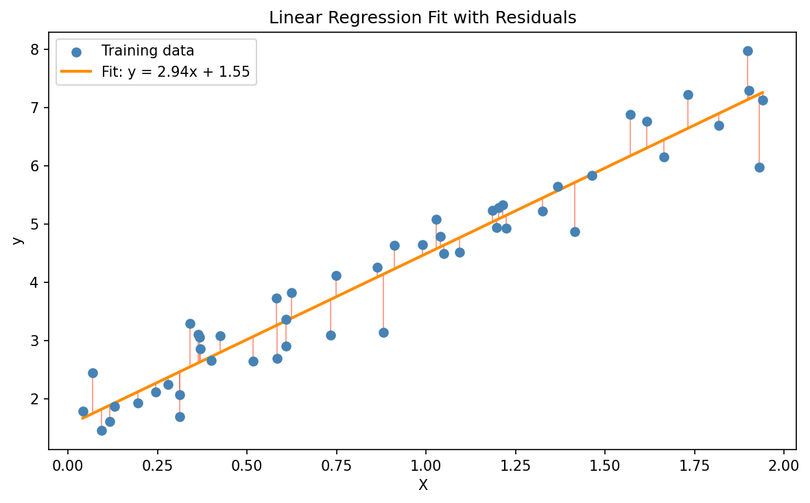
Linear Regression Example

Let’s use linear regression as our example. The model looks like this:

\[\hat{y} = mX + b\]

Where:

• $m$ is the slope (weight)
• $b$ is the Y-intercept (bias)
• $X$ is the input feature
• $\hat{y}$ is the predicted output

$m$ and $b$ are the weights we need to learn. We want to pick values for them so that our predictions $\hat{y}$ land as close as possible to the actual values $y$.

Cost Function

So how do we measure how close our predictions are? That’s what the cost function is for. Here we’ll use the squared error cost function:

\[J(m, b) = \frac{1}{2M} \sum_{i=1}^{M} \left(y^{(i)} - \hat{y}^{(i)}\right)^2\]

Where:

• $M$ = number of training samples
• $y^{(i)}$ = actual value for the $i$-th sample
• $\hat{y}^{(i)}$ = predicted value for the $i$-th sample
• The $\frac{1}{2}$ out front is just there to make the derivative cleaner later on

Our goal is to find $m$ and $b$ that make $J$ as small as possible.

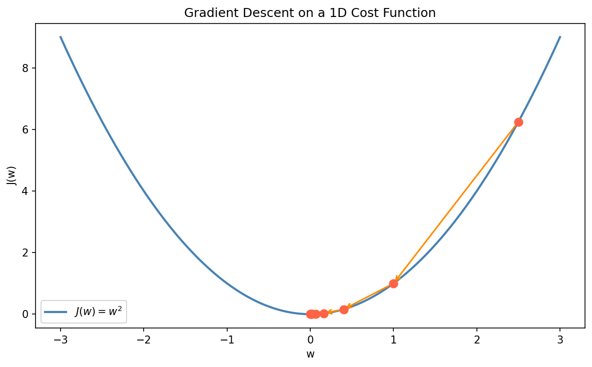
How Gradient Descent Works

Here’s the basic idea. We start with random values for the weights and keep nudging them in a direction that lowers the cost, a little bit at a time:

1. Randomly initialize the weights
2. Compute the gradient, the partial derivatives of the cost function with respect to each weight
3. Update the weights by moving in the opposite direction of the gradient (downhill)
4. Repeat until the gradient is close to zero and we stop moving

The update rule for each weight $w$ looks like this:

\[w := w - \alpha \frac{\partial J}{\partial w}\]

For our linear regression model, the partial derivatives are:

\[\frac{\partial J}{\partial m} = \frac{1}{M} \sum_{i=1}^{M} \left(\hat{y}^{(i)} - y^{(i)}\right) X^{(i)}\] \[\frac{\partial J}{\partial b} = \frac{1}{M} \sum_{i=1}^{M} \left(\hat{y}^{(i)} - y^{(i)}\right)\]

Think of it this way: the gradient is just the slope of the cost surface wherever we currently are. Subtracting it (scaled by $\alpha$) is how we take a step downhill toward the minimum.

Python Implementation

def GradientDescent(X, y, alpha=0.001):
    iteration = 1
    m, n = X.shape
    weights = np.zeros((n, 1))
    Jhist = []
    tolerance = 1e-6

    while True:
        J, grad = costFunction(X, y, weights)
        weights = weights - alpha * grad

        if iteration % 100 == 0:
            print('Iteration #{} — {}'.format(iteration, J))

        if iteration != 1 and abs(Jhist[-1] - J) <= tolerance:
            print('Iteration #{} — {}'.format(iteration - 1, Jhist[-1]))
            print('Iteration #{} — {}'.format(iteration, J))
            print('Converged!!')
            break

        Jhist.append(J)
        iteration += 1

    return weights, Jhist

Two knobs worth paying attention to here:

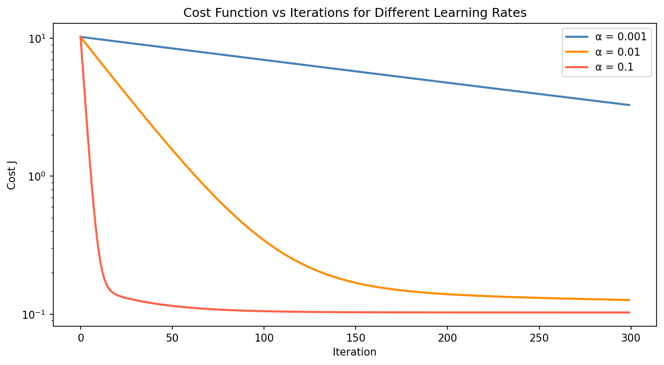
• alpha ($\alpha$) is the learning rate, which controls how big a step we take on each iteration. Pick it too large and the algorithm overshoots and diverges; pick it too small and it takes forever to converge.
• tolerance is the stopping threshold. Once the cost barely changes between iterations, we call it done.

Effect of the Learning Rate

The value of $\alpha$ has a big effect on how fast (and whether) the algorithm converges. Here’s what the cost curves look like for a few different learning rates:

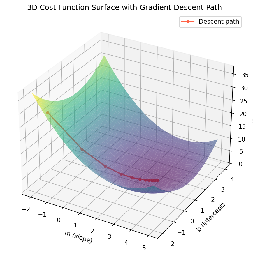
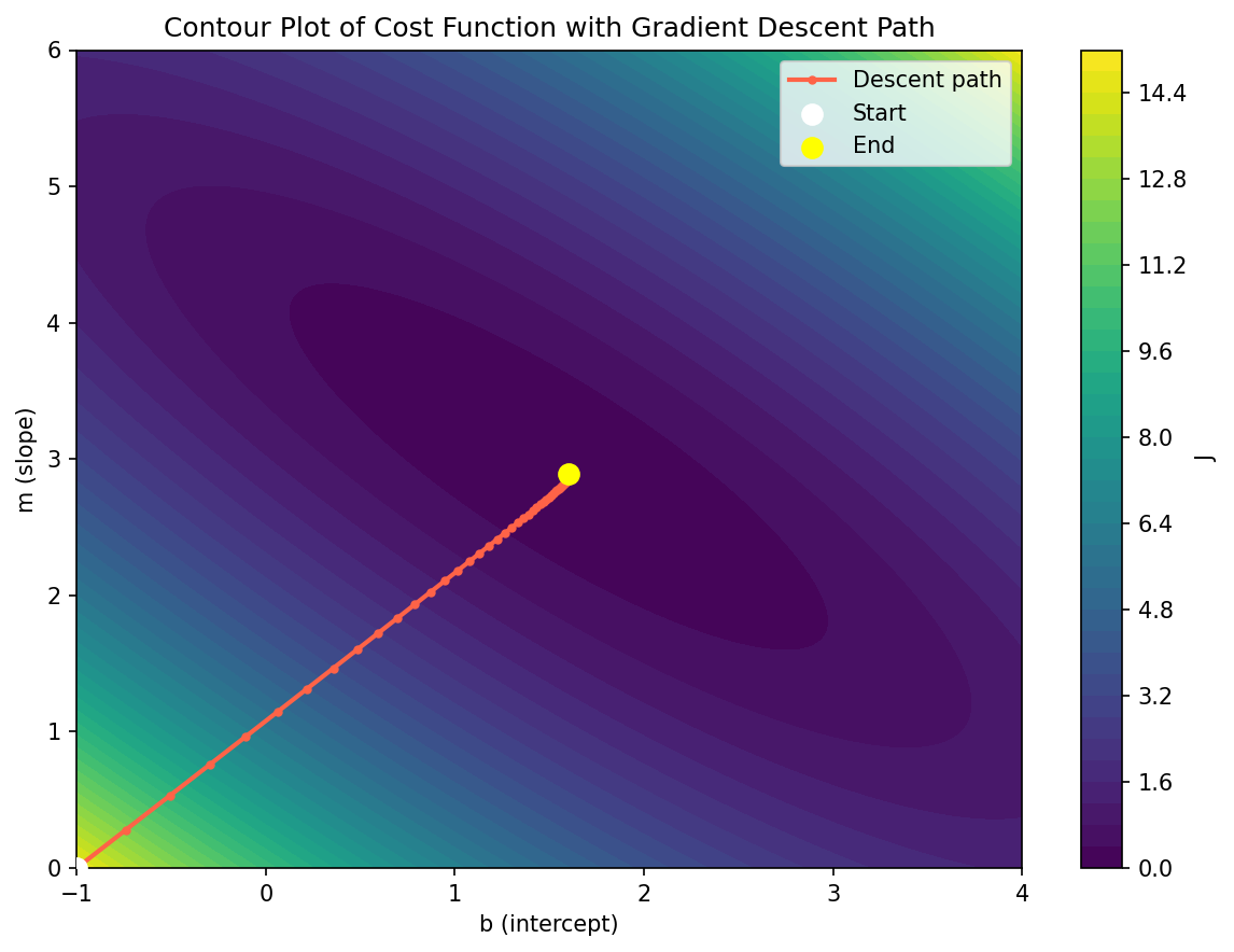
Contour Plot of the Cost Function

Another way to look at the same thing is a 2D contour plot, which shows the path gradient descent takes across the parameter space.

Global vs Local Minima

One catch with gradient descent is that it can get stuck in a local minimum instead of finding the global minimum. Whether that happens depends on the shape of the cost surface and where you started from.

Luckily for linear regression, the squared error cost function is convex, a nice bowl shape with just one minimum. So gradient descent will always find the best solution here, no matter where we start (as long as the learning rate is reasonable).

Things get trickier with deep neural networks, where the cost surface is non-convex and full of local minima and saddle points. That’s where tricks like momentum, adaptive learning rates (Adam, RMSProp), and smarter weight initialization come in.

Key Takeaways

A few things to keep in mind as you play with this:

1. Real-world data is rarely linear. Linear regression is a good starting point, but most real problems need non-linear models.
2. Polynomial regression is a simple extension where you add higher-order feature terms so the model can fit curves instead of straight lines.
3. Batch gradient descent uses the full dataset on every step, which is accurate but slow on large datasets. Stochastic Gradient Descent (SGD) and mini-batch gradient descent are what people actually use in practice, trading a bit of noise per step for much faster iterations.

Gradient descent isn’t just a trick for linear regression. The same idea drives neural networks, SVMs, and pretty much every modern ML algorithm out there, so getting a feel for how it works really pays off once you start debugging your own models.