Simple Perceptron Training Algorithm: Explained
This post was originally published on Medium on July 7, 2018. View original article.
There’s this quote I love from Bill Gates: “I choose a lazy person to do a hard job. Because a lazy person will find an easy way to do it.” That’s honestly how I think about AI. We’re trying to solve some really hard problems, so we look around for the easiest path, and more often than not, nature has already figured it out for us. Humans watched birds and built airplanes. When we wanted machines to think, we looked at the brain.
That’s where artificial neural networks come from. They’re made up of interconnected neurons with synaptic connections, and a typical network has three kinds of layers: input layers that take in the raw features, hidden layers that learn intermediate representations, and output layers that produce the final prediction.
What is a Perceptron?
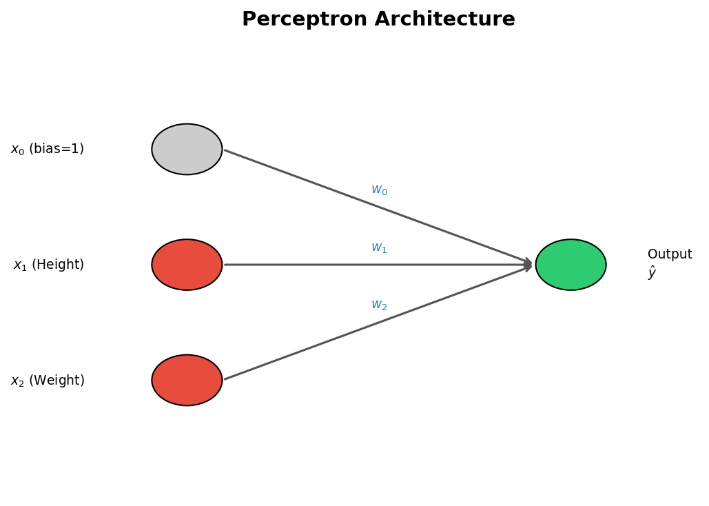
A perceptron is the simplest neural network you can build. It’s basically a computational model of a single neuron. Frank Rosenblatt came up with it back in 1957, and the idea is pretty simple: take one or more inputs, run them through a processor, and spit out a single output. Everything deeper in neural network land is built on top of this.
Classification Problem Example
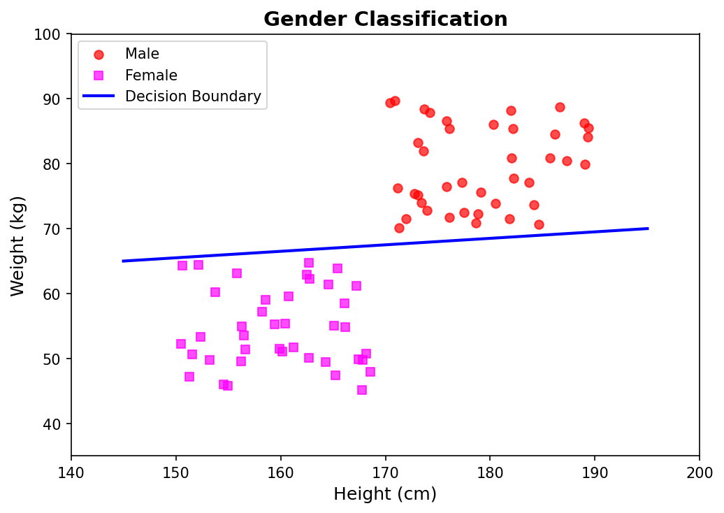
Let’s make this concrete with a gender classification task:
| Feature | Symbol |
|---|---|
| Height (cm) | $x_1$ |
| Weight (kg) | $x_2$ |
| Gender (Male = 1, Female = −1) | $Y$ |
What we want is a decision boundary, a line in the Height–Weight plane that splits the male samples from the female samples.
Mathematical Framework
Line Equation
A straight line in 2-D looks like:
\[ax + by + c = 0\]If we plug in our features, we can classify any point $(x_1, x_2)$ by checking which side of the line it lands on:
- Points above the line give a positive value, so we call them Male ($Y = 1$)
- Points below the line give a negative value, so Female ($Y = -1$)
Vectorized Form
To clean this up, we add a bias term $x_0 = 1$ and stack the weights $w_0, w_1, w_2$ into a weight vector $\mathbf{W}$. Now the decision boundary is just:
\[\mathbf{W} \cdot \mathbf{X} = w_0 x_0 + w_1 x_1 + w_2 x_2 = 0\]Classification Conditions
For a training sample with true label $Y \in {+1, -1}$ and feature vector $\mathbf{X}$, here’s how we tell if we got it right:
| Condition | Meaning |
|---|---|
| $Y \cdot (\mathbf{X} \cdot \mathbf{W}) > 0$ | Correct classification |
| $Y \cdot (\mathbf{X} \cdot \mathbf{W}) < 0$ | Misclassification |
The sign of $Y \cdot (\mathbf{X} \cdot \mathbf{W})$ tells us right away whether the current weights put the sample on the right side of the line.
Weight Update Rule
Every time we get a sample wrong, we nudge the weight vector toward the correct side:
\[\mathbf{W} \leftarrow \mathbf{W} + \eta \cdot Y \cdot \mathbf{X}\]where $\eta$ (eta) is the learning rate, a small positive number that controls how big each step is.
Gradient Descent Derivation
This update rule isn’t something I pulled out of thin air. It falls straight out of doing gradient descent on a pretty natural cost function.
Here’s the per-sample cost:
\[J(\mathbf{W}) = \begin{cases} -Y(\mathbf{X} \cdot \mathbf{W}) & \text{if } -Y(\mathbf{X} \cdot \mathbf{W}) > 0 \quad \text{(misclassification)} \\ 0 & \text{otherwise} \end{cases}\]A couple of things to notice here: $J$ is always non-negative, and it’s only zero when the sample is classified correctly. Which is exactly what we want from a cost.
Partial Derivatives
Now take the gradient with respect to $\mathbf{W}$:
\[\frac{\partial J}{\partial \mathbf{W}} = \begin{cases} -Y \cdot \mathbf{X} & \text{if misclassified} \\ 0 & \text{if correct} \end{cases}\]Gradient Descent Step
The usual gradient descent update is:
\[\mathbf{W} \leftarrow \mathbf{W} - \eta \cdot \frac{\partial J}{\partial \mathbf{W}}\]Plug in the misclassification gradient $-Y \cdot \mathbf{X}$:
\[\mathbf{W} \leftarrow \mathbf{W} - \eta \cdot (-Y \cdot \mathbf{X}) = \mathbf{W} + \eta \cdot Y \cdot \mathbf{X}\]And there it is, the perceptron learning rule, straight out of gradient descent.
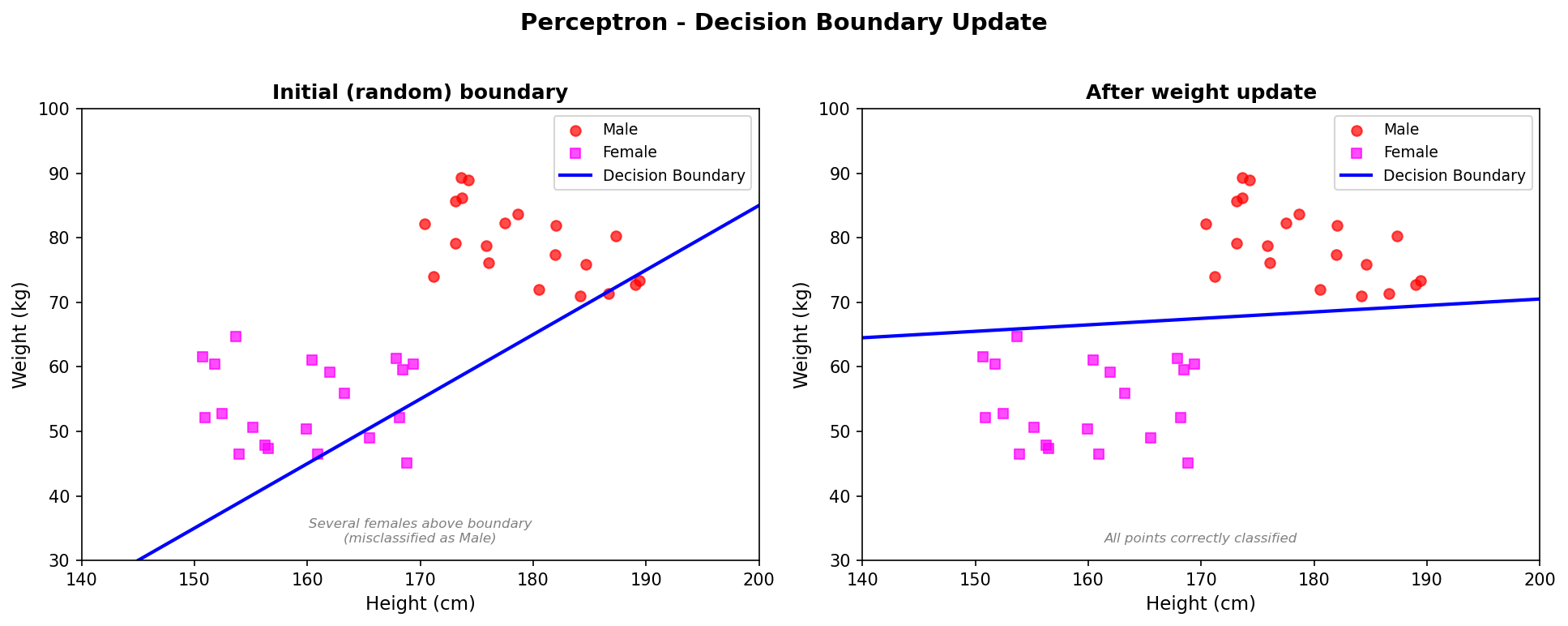
Visualising the Boundary Update
Algorithm Summary
The full training loop is pretty simple:
- Initialise the weight vector $\mathbf{W}$ randomly (or to zeros).
- For each training sample $(\mathbf{X}, Y)$:
- Compute $\hat{y} = \text{sign}(\mathbf{W} \cdot \mathbf{X})$
- If $\hat{y} \neq Y$, update: $\mathbf{W} \leftarrow \mathbf{W} + \eta \cdot Y \cdot \mathbf{X}$
- Repeat over the dataset until nothing is misclassified.
As long as your data is linearly separable, this will converge in a finite number of steps. That’s the perceptron convergence theorem.
Key Limitation
The big catch with perceptrons is that they can only learn on linearly separable data. If you can’t draw a straight line (or hyperplane) between the classes, a perceptron will never converge, it’ll just keep bouncing around forever. That’s the whole reason we ended up with multi-layer networks and non-linear activation functions, which can carve out much more complicated decision boundaries.
You can find a working implementation of the perceptron algorithm, including the scatter plots and training loop, in the accompanying GitHub repository.